Author: Alexandre Kotcherguine, Vision Officer & Investor
Contributors: Georgi Gitchev, Governance Officer & Organisation Domain Lead; Matt Jackson, Growth Officer
This is Article 4 of Phase 1 of the Polity thought-leadership series on go-to-market, capital, and valuation for Web3 infrastructure. It bridges into Phase 2, deriving capital requirements end-to-end through a five-step chain — activation graph → CAC by participant class → infrastructure cost → incentive budget → time-to-critical-mass → capital requirement and burn profile — applied to a generic Web3 infrastructure case. Round size, burn profile, and milestone tranche structure fall out as outputs, not premises. The closed loop from activation strategy to capital requirement is the second of the corpus’s two novelty claims. Article 5 walks one worked operator example through the full chain end-to-end.

TL;DR. Round size for a Web3 infrastructure project is an output of a five-step derivation from the activation graph, not a negotiation against comparables. Burn profile is ramp–plateau–descent, not flat; the regulatory-permission node R_j is the most leveraged single line in the model. Two named failure modes (Comparable-Based Round Sizing, Burn Profile Mismatch) account for the bulk of cohort-observed bridge rounds. The article closes with three falsifiable mechanism hypotheses, sealed at publication, against which the next 18–36 months will produce evidence.
Executive Summary
Synthesis. In this category, failure follows a consistent structure: demand is activated before supply, R_j is treated as a constraint rather than a node to be activated, incentives substitute rather than transition to utility, and capital is sized against comparables rather than the activation path. The result is metric inflation followed by substitution collapse and capital exhaustion.
Most Web3 infrastructure round sizes are not derived from a model. They are reverse-engineered from market comparables, benchmarked against peers at a similar stage, and rounded to a number that reads well on a term sheet. The number is then retrofitted with a milestone narrative, a burn chart, and a bottom-up model that happens to arrive at roughly the same figure.
Investors who have sat through more than a handful of these decks can tell. The tell is that the round size does not depend on any operational variables. Change the activation strategy, change the token design, change the initial jurisdictions, change the subsidy schedule — and the round size stays put, because it was never derived in the first place.
Failure Mode — Comparable-Based Round Sizing.
Condition: round size set by reference to peer comparables and stage benchmarks rather than derived from the project’s own activation graph and activation strategy.
Mechanism: headline round size is fixed first; a milestone narrative and bottom-up model are then constructed to retrofit the chosen number; operational variables (CAC vector, MVNS target, time-to-critical-mass, R_j activation cost per jurisdiction) are calibrated to land on the predetermined total rather than to reflect the actual cost of the activation plan.
Observable symptom: round size does not move when underlying operational variables are perturbed; sensitivity analysis is absent or trivial; experienced infrastructure investors disengage in the first meeting because the quantum is decoupled from the operational thesis.
Cohort prevalence: commonly observed across Web3 infrastructure rounds in the 2021–24 window. The cohort marker is the round-size-as-input retrofit pattern: pitched round sizes cluster narrowly around stage benchmarks regardless of operational thesis variance, and the supporting bottom-up models reverse-engineer to the chosen number rather than producing it.
Bounded applicability: this failure mode is specific to venture-priced rounds. Bank-syndicated rounds (treated in §4.4 below) price on a different mechanism — relative bank balance-sheet allocation rather than peer comparables — and the failure-mode pattern does not transport to that case. The §4 critique applies to venture-priced rounds; bank-syndicated commitment structures are a separate analysis.
Stylised illustration — comparable-based vs derived sizing. Across regulated-finance infrastructure rounds in the 2022–24 window in the named cohort (Methodological Appendix V.3.7.0), comparable-based and derivation-based round sizes for similarly-positioned projects have repeatedly diverged in either direction by 25 to 50 per cent. Where benchmarks were calibrated against larger projects with broader jurisdictional ambition, comparable-based sizes over-shot; the excess showed up as un-targeted incentive emissions, premature multi-jurisdictional onboarding, and elevated burn. Where benchmarks were calibrated against narrower-scope projects, sizes under-shot; teams ran out of capital before MVNS and raised bridge rounds at flat or down valuations. The cohort observation: comparable-based sizing produces a defensible-looking number uncorrelated with actual capital need, with miscalibration scaling in the variance of the project’s thesis from the comparable cohort.
Key Insight. Round size for a Web3 infrastructure project is not a negotiation position. It is an output of a five-step derivation from the activation graph and the activation strategy. Rounds that do not flow from such a derivation are priced on comparables and cannot be defended from first principles.
4.1. The Derivation Chain
Definition — Capital Derivation Chain.
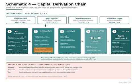
The five-step transformation from a Web3 infrastructure project’s activation graph to its capital requirement: (i) CAC by participant class, multiplied by the MVNS participant-count vector; (ii) infrastructure and operational cost over the runway; (iii) cold-start and post-MVNS maintenance incentive budgets; (iv) time-to-critical-mass; (v) summed and multiplied through to produce round size and burn profile. Each step is a function of the preceding step; none is independently negotiable. The R_j activation cost (Article 1 §1.4) enters the chain at Step (ii) as part of the runway-period operational cost, with magnitude proportional to the jurisdiction count in the activation plan.
Step 1: CAC by participant type
The first input — and the most commonly mishandled — is participant acquisition cost, computed per participant class, not in aggregate. The participant-class asymmetry from Article 1 carries directly into acquisition cost.
Source disclosure for the ranges below. The per-class CAC ranges that follow are vendor-side practitioner estimates calibrated against operator-customer engagements, not cohort observations recovered from the Methodological Appendix dataset. They are presented as order-of-magnitude anchors for the derivation, not as estimates the cohort itself supports. Readers applying the framework to a specific project should substitute calibrated figures from their own operator history or comparable-network data; the derivation chain is the contribution, not the specific anchor values.
In round numbers, using vendor-side practitioner estimates for a generic regulated financial infrastructure network:
· Network Operators (the hard side): tens of thousands to low six figures of dollars per acquisition — legal and regulatory due diligence, substrate licensing and integration, technical onboarding, and account-management time across long sales cycles. Small counts (single digits to low tens), high unit cost, very high retention.
· Service Providers: mid-five-digit dollars per acquisition — regulatory due diligence, integration work, go-live support, and early-period fee rebates. Small-to-medium counts (dozens to low hundreds), high unit cost, high retention.
· Digital Product Merchants: low-five-digit to mid-five-digit dollars per acquisition — product onboarding, listing-fee rebates, distribution support, and per-product compliance review. Medium counts (dozens to low hundreds), medium unit cost, medium-to-high retention.
· End Users (Clients): single dollars to low tens of dollars per acquisition — onboarding incentives, referral rebates, marketing spend. Large counts (tens to hundreds of thousands), low unit cost, variable retention.
Aggregate CAC across these classes is meaningless. What matters is the CAC vector — one number per class — multiplied by the participant-count vector required to reach the minimum viable network state specified in Article 2. The product is the direct acquisition subsidy budget.
For a plausible MVNS of, say, three Operators across two jurisdictions, fifteen Providers, fifty Merchants, and fifty thousand active Clients, a generic worked example lands the direct acquisition subsidy in the low single-digit millions of dollars. The number is not the point; the derivation is. Article 5 walks a different and explicitly hypothetical worked example, with a smaller MVNS and named inputs, for a hypothetical European tokenisation operator; the §4.1 illustrative MVNS above and the Article 5 Operator E case are independent illustrations and should not be conflated.
Step 2: Infrastructure cost (including R_j activation)
Running the network itself costs money, independent of participant acquisition. The infrastructure cost line has four components — three operational and one regulatory.
Core protocol development and maintenance. Engineering payroll or contributor rewards, security audits, bug-bounty programmes, and the long tail of upgrades required to stay current with underlying chains, standards, and regulatory expectations. For a serious project, this runs into seven figures annually and does not taper.
Operational and governance overhead. Treasury management, programme and product oversight, documentation and standards maintenance. Smaller than core development but compounding over the runway.
Infrastructure hosting and third-party services. Identity providers, custody partners, analytics, compliance tooling, node hosting where not self-provisioned. Variable with network volume, but with a meaningful fixed floor.
R_j activation cost — per jurisdiction. Compliance and licensing programmes for each target jurisdiction: regulatory counsel, application and registration fees, capital adequacy commitments where applicable, bilateral discussions with the supervisor, and the calendar time of the Operator’s senior leadership during the licensing window. In the named cohort, this commonly runs to low-six to seven-figure dollars per jurisdiction over 12 to 24 months, depending on regime — lighter authorisations at the low-six to mid-six end, heavyweight authorisations (CSD/MTF, full-stack bank-adjacent licences, systemically-important payment-system designations) at the high-six to mid-seven end. Critically, the R_j line is jurisdiction-additive: jurisdiction j+1 does not amortise against jurisdiction j, because supervisors do not credit each other’s work, and the operator pays the full activation cost again. This is the single most leveraged variable in the model (§4.2 below).
For a generic Web3 infrastructure project, summed over the runway to MVNS, the operational infrastructure components typically run to high single-digit millions; the R_j component, for a two-jurisdiction launch, typically runs to a comparable magnitude on its own.
Step 3: Incentive budget
The incentive budget is where the substitution curve from Article 3 enters the model. It is the capital set aside to pay participants to show up while the utility side of the substitution curve is still too low to retain them unaided.
Two sub-components matter and are worth separating:
Cold-start incentives. These run from launch through MVNS. They include token emissions to early liquidity providers, points programmes for early users, builder grants, and merchant fee rebates. Their size is a function of the bootstrapping loop chosen in Article 2: supply-side-first loops concentrate the budget on operators and merchants; simultaneous loops spread it more broadly.
Post-MVNS maintenance incentives. These run from MVNS to the terminal state where the substitution curve has fully crossed for all participant classes. They are smaller in unit terms but longer in duration. They exist because real networks do not cross the substitution curve cleanly; there is a tail during which incentives still matter, even as utility dominates.
The two components must be tracked separately, because they scale differently with time-to-critical-mass. A longer time-to-critical-mass multiplies the maintenance incentive budget more than the cold-start budget. Misjudging the split understates the total by a large margin. For a generic worked example, the combined incentive budget is commonly the largest single line in the capital requirement — materially larger than direct CAC or infrastructure cost, and often the dominant input.
Step 4: Time-to-critical-mass
Every cost input above is multiplied, implicitly or explicitly, by the time it takes to reach MVNS. Time is the most leveraged variable in the model. Halving the time-to-critical-mass roughly halves the subsidy cost and the incentive maintenance cost; doubling it does the opposite.
Time-to-critical-mass is largely determined by three factors:
The MVNS target itself. A higher bar — more Providers, deeper Merchant coverage, broader Client base — takes longer. The relationship is non-linear: doubling the MVNS target often more than doubles the time, because each later class’s threshold compounds against the depth of all earlier classes.
The activation loop. Supply-side-first loops are typically faster to MVNS in regulated financial infrastructure, because the hard side activates more slowly but the rest of the graph then activates against real utility rather than incentive. Simultaneous loops compress the schedule in well-chosen constrained surfaces, at higher capital cost per unit of time saved. Demand-side-first loops, in infrastructure, usually take longer than projected because the tool-to-network transition consumes time that is not in the original plan.
External constraints — including R_j activation cycles. Regulatory approvals, partnership closings, audit cycles, and market conditions all set floors on how fast the network can activate regardless of internal execution. R_j is the dominant external constraint for regulated infrastructure: in the named cohort, R_j activation cycles of 12 to 24 months per jurisdiction set the floor that no operational acceleration can move below. These floors are legible and should be modelled as hard delays, not contingencies.
A generic time-to-critical-mass estimate for regulated Web3 financial infrastructure is eighteen to thirty months from launch. The range is wide because the inputs are genuinely dispersed; the specific number for a specific project should be defended from its specific MVNS, loop choice, jurisdiction count, and constraint set.
Step 5: Capital requirement and burn profile
With the four preceding inputs, the capital requirement is a computation: sum CAC across participant classes, add infrastructure cost over the runway (including R_j activation per jurisdiction), add both tranches of the incentive budget, multiply the time-sensitive components by time-to-critical-mass, add a buffer for execution variance — typically 25 to 35 per cent for the regulated-finance Web3 category — and the result is the round size. The buffer band is deliberately wider than the conventional 15–20 per cent venture range because the dominant uncertainties (R_j activation cycle slippage, MVNS upper-bound calibration, post-MVNS maintenance tail) carry meaningful probability mass beyond the central case.
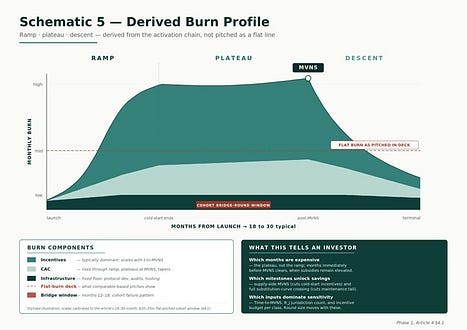
The burn profile follows from the same inputs. It is not flat: it rises through the bootstrapping phase as multiple participant classes are subsidised in parallel, plateaus near MVNS as acquisition costs taper but incentives remain elevated, and descends post-MVNS as the substitution curve crosses and maintenance spend replaces activation spend. A ramp-plateau-descent profile tells an investor which months are the expensive months, which milestones unlock spending reductions, and which variables dominate the sensitivity analysis.
Key Insight. A flat burn projection is not a conservative assumption. It is an unmodelled assumption that the network has no shape.
Stylised illustration — flat-burn deck, ramp-burn reality. A pattern repeatedly observed across regulated-finance infrastructure rounds in the 2022–24 window. Decks pitched flat monthly burn profiles — typically $0.8m to $1.5m monthly over 24 months, totalling $20m to $35m. Twelve to fifteen months in, actual spend was commonly running 30 to 80 per cent above plan, driven by parallel onboarding subsidies during bootstrapping — the ramp the flat model did not price. Bridge rounds at flat or down valuations opened in a substantial share of the cohort to fund the plateau also under-priced. By month twenty-four to thirty, total capital deployed was commonly 30 to 60 per cent above the original round, with dilution costing more than modelling the real shape from the start would have. The flat burn was not an underestimate of magnitude; it was the wrong shape, and the wrong shape was the source of the dilution.
Failure Mode — Burn Profile Mismatch.
Condition: capital plan is built on a flat-burn assumption while real activation produces a ramp-plateau-descent shape.
Mechanism: actual costs concentrate in the bootstrapping ramp and the pre-MVNS plateau (parallel subsidies, accelerated CAC, elevated incentives, R_j activation cycles in flight) rather than spreading evenly; the flat-burn deck under-provisions the peak by 30–60 per cent and over-provisions the descent.
Observable symptom: monthly burn exceeds plan within 6–12 months of launch; team raises an unplanned bridge round at flat or down valuation to fund the plateau the model never priced; total dilution closes 30–50 per cent above what a correctly-shaped initial round would have required.
Cohort prevalence: repeatedly observed across regulated-finance infrastructure rounds in the 2022–24 window (Methodological Appendix V.3.7.0 §8 sets out the per-row support for cohort-level statistics in this article). Across the relevant venture-priced subset of the named cohort, bridge round incidence within 12–18 months of a flat-burn-pitched round of more than $20m has commonly run above half, with bridges sized at 25 to 40 per cent of the original round.
Consequence. A mis-specified capital model does not merely produce inefficiency; it compounds, in this cohort, into irreversible dilution or premature project failure.
4.1. Sensitivity: Which Inputs Dominate
Running the derivation explicitly makes sensitivity visible. Three inputs dominate the capital requirement in almost every generic Web3 financial infrastructure case:
Time-to-critical-mass. Because it multiplies both infrastructure cost and the maintenance incentive budget, it is the most leveraged single input. A six-month delay can easily add twenty to thirty per cent to the total requirement. The implication is that any milestone that accelerates MVNS — a partnership that compresses merchant onboarding, a regulatory approval that unblocks a jurisdiction — is worth a materially higher valuation than its direct revenue impact would suggest.
Jurisdiction count (R_j activation). Because R_j is jurisdiction-additive (Step 2 above), each additional jurisdiction adds its full activation cost to the runway. Moving from one jurisdiction to two roughly doubles the regulatory line item; moving from two to three triples it. Combined with the time-to-critical-mass effect (each R_j activation cycle is 12 to 24 months and these typically run partly serially due to supervisor bandwidth), jurisdiction count is the second most leveraged input. The operational implication is that narrowing the launch surface from three jurisdictions to two often saves more capital than any single operational efficiency the team can find.
Incentive budget per participant class. The product of the CAC vector and the participant-count vector, compounded across the substitution curve, produces a number that dominates the total. Its sensitivity to assumptions about retention and substitution rate is high. A model that shows a realistic, class-by-class substitution schedule is worth more, to an investor, than a model that shows an aggregate subsidy figure twice as big.
The second-order inputs — core infrastructure cost and direct Client acquisition cost — matter but do not dominate.
A worked sensitivity, using the §4.1 illustrative MVNS as the baseline (three Operators across two jurisdictions, fifteen Providers, fifty Merchants, fifty thousand active Clients), gives a directionally indicative round-size response to three perturbations. (Article 5 walks the same sensitivity for one specific worked operator example with named inputs, and on a different — smaller — MVNS specification.)
· A six-month slip in time-to-critical-mass (24 to 30 months) propagates through both infrastructure cost and the maintenance portion of the incentive budget; the round size rises by approximately twenty per cent.
· Narrowing the launch surface from two jurisdictions to one removes one Operator, removes one R_j activation cost line, reduces Provider and Merchant counts proportionally, compresses cold-start incentives, and shortens time-to-critical-mass through fewer regulatory dependencies; the round size falls by approximately twenty-two to twenty-five per cent.
· A twenty per cent increase in the per-class CAC vector lifts both direct acquisition costs and the cold-start portion of the incentive budget but does not affect maintenance incentives or infrastructure cost; the round size rises by approximately six per cent.
4.2. Milestone-Based Tranching
The burn profile, once derived, naturally suggests a tranched rather than single-tranche round structure. The argument is straightforward. Capital is drawn down according to a ramp-plateau-descent profile, with MVNS as the decisive inflection point. Releasing later capital against achievement of earlier milestones is both more efficient and more aligned.
A typical structure for a generic Web3 infrastructure project might be: an initial tranche covering bootstrapping through an early MVNS checkpoint (typically R_j active in jurisdiction one and supply-side at half-MVNS); a second tranche, contingent on that checkpoint, covering the plateau and the approach to full MVNS; a final tranche covering the descent and post-MVNS maintenance. The precise triggers and sizes depend on the derivation; the principle does not.
Milestone tranching does two things at once. It reduces the blended cost of capital, because later tranches are priced against more evidence. And it imposes discipline: each milestone is defined against the derived burn profile, not against narrative targets, so progress against the plan is legible and auditable.
4.3. Capital Market Reality and the Fundable Round
The derivation produces what the project needs. The market produces what the project can raise. The two are not always the same. A complete capital model treats market constraints as first-class inputs alongside the operational ones.
Pricing constraints. The valuation a project can defend at the moment it raises is bounded by the market’s category appetite, the project’s evidence base, and recent comparable exits. A derivation that calls for $30m at a $150m post may, in a cooler tape, only be fundable at $20m at $100m post — or at $30m at $80m post. The derivation is unchanged; the price has moved.
Timing constraints. Capital availability for regulated Web3 infrastructure is cyclical. Windows open and close on a horizon of months. The activation plan’s milestone structure must be readable at the speed the market closes a round — typically eight to twelve weeks in a normal tape, four to six in a hot one, indefinite in a closed one. A derivation that requires a six-month diligence cycle to be understood is, in practice, unfundable in any window narrower than that.
Investor-appetite constraints. Specialist infrastructure investors have finite cheque-size ranges and finite category allocations per fund. A $45m requirement may be fundable only as a syndicate of three; a $5m requirement may be too small for the only specialists who could underwrite the diligence. Both cases require the derivation to bend toward what the cap table can plausibly assemble, without bending the operational plan with it.
Bank-syndicated rounds — a separate pricing mechanism. By total external capital raised, the largest-funded members of the named cohort (Methodological Appendix V.3.7.0) — Digital Asset / Canton Network (most recent strategic round $135m, June 2025, led by DRW Venture Capital and Tradeweb Markets, bank participation including BNP Paribas and Goldman Sachs); Fnality International (Series B £77.7m / ~$95m, November 2023, led by Goldman Sachs and BNP Paribas; Series C $136m / £99.7m, September 2025, led by WisdomTree, Bank of America, Citi, KBC Group, Temasek and Tradeweb; ~24 named shareholder institutions of which 16+ are banks); R3 (Series A $107m, May 2017, with 40+ institutional investors including most G-SIBs and Intel) — were sized via syndicates dominated by financial institutions and infrastructure-aligned strategics rather than by traditional venture-priced rounds. Per-round source citations are in the Methodological Appendix V.3.7.0. These rounds price on a different mechanism: relative balance-sheet allocation among participating institutions, with each slice a function of strategic interest and category-defensive infrastructure budget. The Comparable-Based Round Sizing failure mode does not apply to this commitment structure — the comparables are other institutions’ commitments, not other projects’ rounds, with different failure modes (consortium-design risk, free-rider dynamics among non-leading participants, slow pace of fully-syndicated close). The §4 critique applies to venture-priced rounds; institution-syndicated rounds are a Phase 2 subject.
Note on the §4.4 references. The funding figures above are reported for analytical context, anchored to specific named press releases and shareholder-list disclosures by the projects themselves; they are not reported as a competitive ranking. Polity is an infrastructure substrate vendor; the named projects are operating networks. The two are not competitors in the sense relevant to comparative-advertising regulation, and the analytical use of named-project figures here is a public-record reading rather than a benchmark of competitor performance.
Reconciling the operational and market views. When the derived requirement and the fundable reality diverge, the response is not to retrofit the model. It is to surface the gap and choose, on the operational side, what the smaller round actually buys: a narrower initial surface, a delayed jurisdiction (deferring R_j activation in j+1), a deferred Provider class. Each compresses the derivation and produces a smaller defensible number. The discipline is that the operational concession is visible, and the smaller round is still derived — just from a constrained version of the activation plan.
4.4. Why This Matters for the Round
Two implications follow for any live round.
The conversation with investors changes shape. Instead of defending a number, the team defends a model. The number becomes an output. Investors with deep infrastructure experience recognise the difference within the first meeting; those without it either engage with the model or self-select out.
Capital allocation discipline becomes possible. When the round size is derived from the operational variables, changes to those variables are first-class inputs. A decision to narrow the initial launch surface, defer a jurisdiction (defer R_j in j+1), or accelerate a partnership flows directly into an updated capital requirement. The treasury becomes a function of the activation plan, not a fixed constraint — a topic taken up in Phase 2.
4.5. Explanatory Coverage and Falsifiable Hypotheses
An analytical framework is only as good as the work it does on cases. This section splits that work into two parts: explanatory coverage of the existing named cohort (§4.6a), and falsifiable hypotheses about projects not yet in the cohort (§4.6b). The two are different epistemic claims and are stated separately rather than as one. The retrospective claim is about the framework’s coverage of evidence already in hand; the prospective claim is a bet on evidence the next 18 to 36 months will produce.
4.6a Retrospective — explanatory coverage of the named cohort
Of the fifteen projects in the named cohort documented in the Methodological Appendix V.3.7.0 (with Provenance Blockchain moved to the inclusion-exception list, leaving fourteen substantive cohort members for explanatory analysis):
· Subsumed under the framework’s mechanisms (eleven of fourteen): the cohort members whose observed activation difficulty, recapitalisation, or pivot maps onto one of the framework’s named mechanisms — supply-side mis-sequencing (the demand-first L1 thesis cohort), regulatory mis-pacing (Polymesh, SDX, Fnality’s four-year cycle), substitution-curve failure (the token-incentivised members), comparable-based round sizing (the venture-priced L1s in the cohort), or burn-profile mismatch.
· Explained by adjacent mechanisms the framework names but does not formalise (two of fourteen): the MANTRA OM token collapse of April 2025 is more accurately a token-distribution / exit-liquidity event than a substitution-curve collapse (Article 3 boundary note); the VMware Blockchain row (the November 2023 Broadcom-acquisition discontinuation) is closer to Rival 4 (tokenisation didn’t reduce settlement costs enough) than to a graph-sequencing failure, with the widely-cited ASX-CHESS termination separately attributed to the Digital Asset / DAML programme with VMware as infrastructure partner from 2019 (per Article 1 §1.6 and the cohort dataset row). Both cohort rows are flagged in the Appendix as failure modes outside the framework’s core scope rather than as supportive evidence of mechanisms the framework formalises.
The framework’s current specification under-covers (one of fourteen): the Hedera Hashgraph case under its Council governance model is one the framework does not fully cover at Phase 1. The activation-graph view treats Capital Contributors as off-graph and assumes the Operator’s treasury is the principal source of pre-MVNS subsidy. The Hedera Council structure combines features the framework treats as separate: Council members are described in public sources as capital contributors, governance principals, and the regulated counterparties whose participation is the network’s value proposition. With Council fee revenue (a recurring distribution back to participants from network-fee receipts) and named-corporate Council membership, the capital-contributor class and the supply-side participant class are the same parties, and the substitution curve for that combined class is underspecified. A future revision may extend the framework with a “fused-class” specialisation or concede that Council-governed networks sit outside its scope. As of V.3.7.0, no such specialisation exists; the right Phase 2 question is whether one extension covers Council-governed and bank-syndicated members (§4.4) together. This is a comment on framework coverage, not on the strategy or prospects of any named cohort member.
This is explanatory coverage, not prediction. The framework was built knowing the cohort; coverage of the cohort is therefore the lower bound, not the upper bound, of what the framework can claim. The next subsection states what the framework claims about cases it does not yet know.
4.6b Prospective — locked research hypotheses, sealed at publication
As of the publication date of this article (26 May 2026, V.3.7.0), the framework states the following research hypotheses about Web3 infrastructure projects raising rounds in the twelve months from publication. Each hypothesis names a horizon, a measurable threshold, and a counter-evidence condition. The cohort against which these hypotheses are tested is locked at publication: it consists of any Web3 infrastructure project meeting the Methodological Appendix V.3.7.0 inclusion criteria and raising a primary round between publication date and 26 May 2027. A re-pull will be published at the 12, 18, and 24-month horizons, listing the qualifying projects and their observed outcomes against each hypothesis, regardless of whether the hypotheses hold. Full resolution of the hypothesis set runs through May 2029 (24 months past the close of the raise window).
Regulatory status of this section. The hypotheses below are stated for falsification — so the framework can be shown wrong by future evidence — not as investment recommendations, financial promotions, or solicitations. They are not directed at retail investors and are not advice on any named entity. They are framework claims about category-level patterns, testable against the locked cohort.
Hypothesis 1 — sequence (18 to 24-month horizon).
The framework’s hypothesis is that a regulated-finance Web3 infrastructure network raising ≥$10m primary capital between 26 May 2026 and 26 May 2027 that activates demand (Clients) before its supply side (Operators / Providers / Merchants) reaches MVNS will, within 18 to 24 months of mainnet launch, exhibit at least one of: (a) a weekly-active-participant figure that has decayed by ≥ 70 per cent from its peak, (b) a bridge round at flat or down valuation, or © a publicly-disclosed strategic pivot away from the original thesis.
Counter-evidence: a network sequenced this way that, at month 24, holds > 50 per cent of peak weekly actives without a bridge round and without thesis revision.
Hypothesis 2 — substitution (6-month horizon from first emission step-down).
The framework’s hypothesis is that a token-incentive programme launched between 26 May 2026 and 26 May 2027 without a per-class substitution-curve design will, within six months of the first scheduled emission step-down, lose at least 50 per cent of the participation acquired during the emission peak, on a per-class basis for at least one class.
Counter-evidence: a programme that retains > 60 per cent of peak per-class participation through two consecutive scheduled emission step-downs.
Hypothesis 3 — burn shape (12 to 18-month horizon).
The framework’s hypothesis is that, among regulated-finance infrastructure projects raising rounds of > $20m on a flat-burn capital model between 26 May 2026 and 26 May 2027, ≥ 50 per cent will, within 12 to 18 months of round close, raise an unplanned bridge round, with the bridge size averaging between 25 and 40 per cent of the original round.
Counter-evidence: a cohort that achieves its 18-month milestones on the original capital plan without recourse to bridge financing.
A fourth meta-hypothesis previously stated at this point — concerning the relative valuation of operators publishing an explicit derivation against those that do not — has been retired in V.3.7.0. The hypothesis was self-interested (Polity’s framework would expect adopters of its framework to outperform), rested on a small denominator, and characterised market valuation outcomes for an identifiable sub-cohort in a way that risked reading as a financial promotion. The substantive observation — that derivation publication is correlated with diligence-cycle outcomes — is moved to Phase 2, where it can be addressed inside the Investor Readiness frame the Disciplined Fundraising series already provides.
Each hypothesis names a horizon and a measurable threshold. Failures to observe the predicted patterns will be taken as evidence the framework is wrong, not as occasions to retrofit the framework. The Phase 2 series will revisit these hypotheses on a rolling basis as the market produces evidence.
Posture commitment. Hypotheses 1–3 are mechanism-grounded claims of the framework, stated with horizons, thresholds, and counter-evidence conditions because that is what makes them falsifiable. Polity will publish the result of the re-pull at 12, 18, and 24 months whether or not the hypotheses hold. A framework that does not commit cannot be wrong; a framework that does, and is, becomes information about the world. The hypotheses are not advice on, or characterisation of, any specific named entity’s prospects.
Methodological note
Empirical illustrations and quantitative ranges are stylised and synthesised from publicly observable patterns across the named cohort (Methodological Appendix V.3.7.0); they describe no specific entity. Sensitivity figures (§4.2) are illustrative against a generic baseline, not project-specific. Per-class CAC ranges (§4.1 Step 1) are vendor-side practitioner estimates per the inline source note, not cohort-derived. §4.4 funding figures are anchored to named press releases and shareholder lists; full citations are in the Methodological Appendix V.3.7.0.
Principle — Round Size as Derivation, Not Negotiation.
The capital requirement of a Web3 infrastructure project SHALL be derived from its activation graph and activation strategy through an explicit derivation chain. Round sizes that do not reduce to this derivation — whatever their market-comparable justification — are not defensible from first principles and should not be treated as financially disciplined.
Constraint — Competitive Disclosure Discipline.
Where the derivation methodology is disclosed for credibility (as in this article), project-specific derivation outputs — MVNS targets, participant-class CACs, jurisdictional timing assumptions — for live operator-customers SHALL NOT be disclosed in the same vehicle. The method is public; the calibration is not.
Note: this constraint applies to live operators. Didactic worked examples on hypothetical operators (such as Operator E in Article 5) are explicitly out of scope for this constraint, because the derivation outputs in such examples reveal nothing about a real operator’s plan. The constraint binds in published material about Polity’s actual operator-customers, none of whom are described in this corpus.
Closing
The derivation chain — activation graph → CAC → infrastructure (with R_j) → incentives → time → capital — is the bridge between the operational and financial models of a Web3 infrastructure project. The quality of each derived number — round size, burn profile, milestone structure — is no better than the quality of the activation graph underneath. This is the reason Phase 1 opened with the activation graph rather than with capital, and why the closed loop from graph to round size is one of the corpus’s two principal novelty claims.
Next: Article 5 walks one worked operator example end-to-end through the framework, from graph to round size. Phase 2 of this series (beginning July 2026) connects the derived round size to the Investor Readiness Framework set out in the Disciplined Fundraising series — opening with Model-Driven Fundraising on how a derived requirement shapes the round itself: size, tranche structure, instrument choice, and investor composition.
Disclaimer
This article is published for informational and educational purposes only. It does not constitute investment, legal, tax, or financial advice, an endorsement of any product or security, or any offer or solicitation. References to named projects in the cohort and to named public events (token launches, recapitalisations, discontinuations, regulatory milestones) are factual public-record observations recorded for analytical purposes; they are not assessments of those projects’ merits or prospects, and the framework expresses no view on the future trajectory of any individual project. Readers should conduct their own due diligence and consult qualified professionals before acting on any of its content.
Polity is a B2B technology vendor that develops substrate infrastructure for the operators of regulated digital finance networks. Polity does not provide investment advice, custody, crypto-asset services under Regulation (EU) 2023/1114 (MiCA), or any other regulated activity; operator-customers are the regulated entities for any service delivered on Polity substrate. Polity has a commercial interest in the adoption of this framework (operator-customers typically build on Polity substrate); this conflict of interest is disclosed for transparency and is not cured by it.
Forward-looking statements in this corpus — including the §4.6b research hypotheses — are based on current expectations and may prove materially incorrect. Past cohort patterns are not a guarantee of future outcomes. The §4.6b hypotheses are stated for falsification, not as investment recommendations, financial promotions, or solicitations within any applicable regulatory regime.
Published from the European Economic Area; not directed at any person in a jurisdiction where its publication would be contrary to local law. This corpus is not a marketing communication relating to any specific crypto-asset within the meaning of Article 27 of Regulation (EU) 2023/1114 (MiCA); it is a category-level analytical framework. Personal data of natural persons (typically corporate officers of named cohort projects) is processed under legitimate-interest grounds (GDPR Article 6(1)(f)) and confined to the public commercial record.
Third-party names and sources are public-record events; their inclusion implies no commercial relationship, endorsement, partnership, or affiliation. Characterisations of causes, mechanisms, or outcomes of named cohort projects are this framework’s analytical interpretation of the public record, not statements of fact about any entity’s strategy or condition. Inclusion in the companion Methodological Appendix implies no commercial relationship.
References
(1) Gornall, W. and Strebulaev, I. (2020). ‘Squaring Venture Capital Valuations with Reality.’ Journal of Financial Economics, 135(1), pp. 120–143. Available at: https://doi.org/10.1016/j.jfineco.2018.04.015
(2) OECD (2022). Why Decentralised Finance (DeFi) Matters and the Policy Implications. OECD Working Paper. Available at: https://doi.org/10.1787/109084ae-en
(3) Bank for International Settlements (2023). ‘The Crypto Ecosystem: Key Elements and Risks.’ BIS Report to the G20 Finance Ministers and Central Bank Governors. Available at: https://www.bis.org/publ/othp72.htm
(4) Polity (2026). Phase 1 Methodological Appendix and Cohort Dataset, V.3.7.0. Polity Thought Leadership Series, Phase 1, companion artefact.